Useful Things Described by the Normal Curve

The normal curve is symmetrical 2. It has the following properties.

The Normal Distribution Sociology 3112 Department Of Sociology The University Of Utah

The normal distribution is the most commonly-used probability distribution in all of statistics.

. A density curve is scaled so that the area under the curve is 1. The characteristics of the normal curve are applied in statistics in the process of establishing the probability of an event occurring. A normal curve summarizing the percentages given by the empirical rule is below.

This probability method plays a crucial role in asset return calculation and risk management strategy decisions. The center line of the normal density curve is at the mean μ. The normally distributed curve should be symmetric at the centre.

Marks on a test. Height of the population is the example of normal distribution. This is not just any distribution but atheoretical one with several unique characteristics.

The area is greatest in the middle where the hump is and thins out toward the tails. The change of curvature in the bell-shaped curve occurs at μ σ and μ σ. The normal distribution should be defined by the mean and standard deviation.

It is always symmetrical with equal areas on both sides of the curve. Most people recognize its familiar bell-shaped curve in statistical reports. Size of things produced by machines.

The area under the whole curve is one. The mean of the distribution determines the location of the center of the graph and the standard deviation determines the height and width of the graph and the total area under the normal curve is equal to 1. We say the data is normally distributed.

The maximum ordinate occurs at the centre 5. The mean µ and the standard deviation σ. A normal density curve is a bell-shaped curve.

A normal distribution resembles an asymmetric arrangement of most of the values around the mean such that the curve so formed looks like a bell. Third the normal curves standard deviation tell us what percentage of observations fall within a specific distance from the mean. The normal distribution curve must have only one peak.

The empirical rule says that for any normal bell-shaped curve approximately. The normal distribution or bell curve is most familiar and useful toteachers in describing the frequency of standardized test scores how manystudents earned particular scores. About 68 of data falls within one standard deviation of the mean.

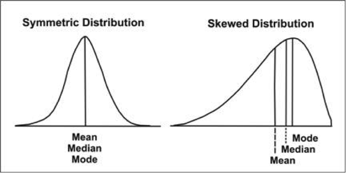
It makes sense that the area under the normal curve is equivalent to the probability of randomly drawing a value in that range. Both are located at the center of the distribution. That is for the normal curve all measures of central tendency fall on the same value.

It has two key parameters. Second the normal curve is centered on the mean which also happens to be equal to its median and mode. Normal distributions comprise of all set of values from one variable with a display made in a histogram.

Normal distribution is a bell-shaped curve where meanmodemedian. The normal curve is unimodal 3. The data being described are the verbal SAT scores for all seniors taking the test one year.

When we have a normal curve the area below the curve. Unimodal it has one peak Mean and median are equal. Many things closely follow a Normal Distribution.

997of the values data fall within 3 standard deviations of the mean in either direction. From the figure above about 68 of seniors. The main thing to realise about the Normal curve is that the aspect which is easiest to interpret quantitatively is not the height of the curve but the area under the curve.

Since this is describing a population we will denote the mean and standard deviation as m 490 and s 100 respectively. The area under the curve up to a given value is the proportion of the population which has values smaller than the given value. The z-scores are used to establish the number of standard deviations a variable is from the mean.

68of the values data fall within 1 standard deviation of the mean in either direction. There should be exactly half of the values are to the right of the centre and exactly half of the values are to the left of the centre. 7 Characteristics of Normal Curve STUDY Flashcards Learn Write Spell Test PLAY Match Gravity Created by Samantha_Hemsworth Terms in this set 7 1 Never touches X 2 BellShaped 3.

If you plot the probability distribution curve using its computed probability density function then the area under the curve for a. The normal curve is asymptotic to the X-axis 6. That is consistent with the fact that there are more values close to the mean in a normal distribution than far from it.

Mean median and mode coincide 4. The normal distribution is a continuous probability distribution that is symmetrical around its mean most of the observations cluster around the central peak and the probabilities for values further away from the mean taper off equally in both directions. The normal distribution curve can be divided in half with equal values falling on either side Of the most frequently occurring value Indicates random or chance variation The peak of the normal distribution curve represents the center of the process They are divided up into 3 standard deviations on each side of the mean.

95of the values data fall within 2 standard deviations of the mean in either direction. Lets understand the daily life examples of Normal Distribution. A normal distribution is described by a normal density curve.

The Normal Distribution has. Mean median mode Coincide at one point at the center of the curve they have equal value Mean standard deviation Two parameters used to describe normal curve Probability Areas under the normal curve indicate Standard score Distance of the score from the mean in terms of the standard deviation Standard score. The height of the curve declines symmetrically and.

The Normal Curve Boundless Statistics

The Normal Distribution Table Definition

The Normal Curve Boundless Statistics

The Standard Normal Distribution